Self Study Projects

2022, Jan 01    

Self Study Projects

The projects contained within this webpage relate to various topics that I have deemed interesting and wanted to enhance my knowledge and apply what I leanred in a practical capacity. These projects were created to further my perosnal education and profesional development and serve as a medium for showcasing my skills outside of structured learning.

• Each project file will be in the “Appendix” section located at the bottom of the webpage.

Discounted Cash Flow Model

This project was conducted voluntarily to practice my company valuation and Microsoft Excel skills. My goal for this project was to create a full functioning dynamic Discounted Cash Flow Model completely from scratch and to showcase my financial and accounting literacy to potential employers.

Files included:

• DCF Model Excel File

Brookfield Energy Partners Corp. was selected as the company to be evaluated. This company sits in my personal portfolio and is an excellent energy holdings company with sufficient historical data for analysis. I used the annual reports from 2018 - 2020 to provide the financial data from their income statements and balance sheet. I will provide a summary of each step of the model and my thought process during these specific steps.

Data

To provide a detailed Discounted Cash Flow Model for evaluating a company’s future value, you will need data from the income statement to calculate revenue growth rates and weighted average cost of capital, and data from the balance sheet for calculating net working capital and capital expenditures. After finding the annual reports from Brookfield’s website, you need to copy it over to your sheet to be used in the model’s formulas.

The earnings report for Q4 2021 was not released during the time I drated this model. Q1 - Q3 2021 data was used to help project 2021’s final values. I used a simple average growth rate to calculate 2021’s ending values. With these values provided, you can now move into constructing the model.

WACC

For the DCF Model, you must calculate the Weighted Average Cost of Capital for the terminal value calculation. CAPM or Capital Asset Pricing Model is the method used for finding the cost of equity for BEPC. The inputs needed are the Risk-free rate which is usually the 10-Year Treasury yield, the beta of the stock which can be found on different financial websites that monitor share price movements, and the expected market return which is the projected return of the overall stock market for that year.

• Cost of Equity Formula: = Expected Market Return + Beta * (Expected Market Return - Risk-free Rate)

The next part of the WACC is the cost of debt. To calculate the cost of debt, look at the outstanding notes that the company has issued and use a simple average of all interest rates for those notes to find the cost of debt.

• Cost of Debt Formula = Average of all interests rates of outstanding notes

After you have the cost of equity and cost of debt, use these values in the WACC formula to produce the Weighted Average Cost of Capital value.

• WACC Formula = ((% of Equity * Cost of Equity) + (% of Debt * Cost of Debt) * (1 - Tax Rate))

The final step in this section is finding the terminal growth rate. To calculate “TGR”, you can use average inflation values from the last three years along with growth of GDP in the same time frame.

• Terminal Growth Rate = Average of (mean inflation rate & mean GDP growth rate for the same period of time)

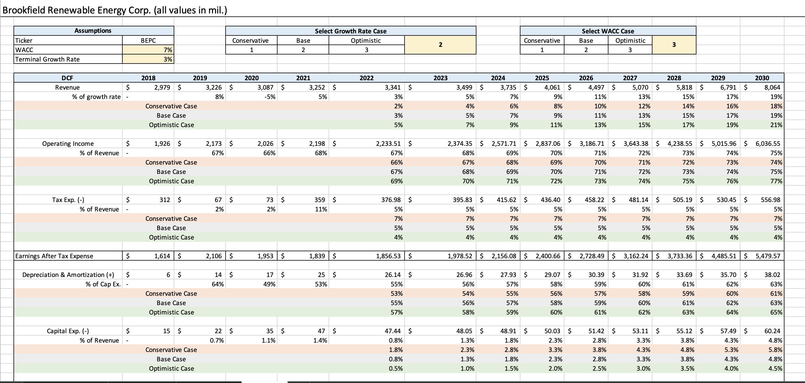
In the model, there is a base, optimistic and conservative case for each of the main components of the WACC. This was constructed to allow a dynamic model that can be altered to test different assumptions about the overall market, specific company risks or the analyst’s own expectations.

Projections

The DCF model is useful for determining the company’s stock price in the future by discounting cash flows back to present value. In order to perform the analysis, project the revenues of the company out five or ten years. This particular model projects until 2030 which equates to nine years of forecasts. Using the data from the annual reports, you can project the revenues and calculate “Earnings After Tax Expense” for that year. You are left with income that hasn’t accounted for depreciation or the changes in non-cash assets and liabilities.

“Depreciation & Amortization” is added back to the income because these are non-cash expenses accounted for on the income statement. “Capital Expenditure” (or CapEx) is usually a portion of the depreciation expense because this expense is usually attributed to a purchase of large machinery, equipment or buildings that are expensed through the useful life of that working asset. “Net Working Capital” is the current assets less cash minus the current liabilities less debt. This is to account for the net increase of assets that are not cash and they cannot be included as these assets are not producing any cash flows at the moment of accounting.

Once these values have been estimated, they can be included in the formula for unlevered cash flow. Each year in the model now produces a free cash flow value.

Present Value

The model now has nine cash flow values all the way until 2030. However, these values need to be discounted back to the present value by using the WACC value. Using the cash flow value and then multiplying it by one plus the WACC to the power of the current year, you find the present value of that cash flow.

To calculate the present value of the enterprise, you must multiply the projected cash flow in 2030 by one times the WACC value then divided by the WACC minus the terminal growth rate to find the terminal value of the enterprise.

After this calculation, you will use the terminal value multiplied by one times the WACC value of the ninth year of the projection. This calculation will provide the analyst with the discounted value of the entire enterprise.

Share Price Calculation

To find the intrinsic value of the share price, first sum all of the present value of each year’s cash flow. From this, you will find the enterprise value of the free cash flows. Once you have this value, add back the cash, minus the debt, and you get the equity value of the cash flows. Divide the equity value by the shares outstanding and you will find the intrinsic value of the share price. This model allows for the analyst to evaluate a share’s price based on the company’s cash flows and determine if the current price is too expensive or is cheap compared to the intrinsic value of the company.

The model is completely dynamic with the base, optimistic and conservative case toggle table at the top of the sheet to allow for different hypotheses to be tested. This model is not an “exact science” but it provides useful information when determining the true value of specific companies. These models can be developed further than what was showcased in this project or can even be simplified for faster and more efficient analysis. It depends on the needs of the analyst and the assumptions that will be included within the model.

Leveraged Buyout Model

The Leveraged Buyout Model is an important model to construct for Private Equity firms as this allows the firm to project the return on investment of the private company they intend to acquire. Private Equity is a field that I am highly interested in learning about and thus learning how to develop a LBO Model is essential for being an Private Equity analyst. This model also provides further practice in financial and valuation concepts.

Files included”

• LBO Model Excel File

Assumptions

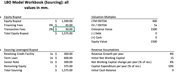
The “Assumptions” tab outlines the prompt for the model. The key elements to account for range from the “Enterprise Value” to the various financial metrics that will be consistent throughout the projections. All the assumptions stated allow the analyst to build an accurate and in-depth LBO Model and even allow for dynamic toggling to test different inputs and calculate various outputs.

Sourcing

The “Sourcing” tab outlines all assumptions in their numerical value so the analyst can use them in the model’s formulas. In Private Equity, firms tend to issue different debt instruments to finance the acquisition. In this model, the debt being used is a “Revolving Credit Facility, Term Loan, and Senior Note.” There is also “Financing and Transaction fees” associated with the acquisition deal, being 3% and 2% of “Enterprise Value,” respectively. This gives you the full “Equity Value” that must be accounted for when purchasing the private company.

Key Elements

• Revolving Credit Facility: A financial instrument that allows the borrower to repay or borrow from the credit line at different points in its useful life. This provides the borrower greater flexibility in using the debt to finance their operations or acquisitions.
• Term Loan: A loan that is given in lump sum to the borrower under specific terms from the lender.
• Senior Note: A bond that is issued from the company looking to raise capital and is repayed in full at the end of the useful life of the bond. These bonds come with a coupon that is paid out to the lender, usually at the end of each year.
• Remaining Equity: The difference between the “Equity Value” and the sourced debt is paid for in equity from the purchasing company.

Debt Schedule

The “Debt Schedule” tab is the most intergral part of this model as it outlines the projections for paying off all the oustanding debt used in financing the acquistion. This allows the analyst to determine when the firm can have an optimal exit after all debt is paid off.

Key Elements

• LIBOR: The “London Interbank Offered Rate” is used as a benchmark for interest rates in outstanding debt in the global capital markets. The model uses a simple 1% assumption across all years to make calculations manageable.
• Spread: The spread on the outstanding debt instruments is calculated with U.S Treasury bond yields and corporate bonds with the same maturity length. It can determine the risk associated on that specific corporate bond. U.S. Treasury bonds are seen as “risk-free” and the difference on the two bonds’ yields can indicate safe or risky investment. The spread is 3% for the all debt instruments.
• Mandatory Amortization: This value references the mandatory repayment of the loan’s principal that must be paid out on the negotiated date in the year. Amortization is 10% for all years in the projection.

After calculating the repayment schedule for all the debt, the model can show you the total interest payment which can help the firm determine future free cash flows of the acquisition.

Projections

The “Projections” tab outlines the logical progression of calculating the value of the acquisition after each year of holding. It requires a projected “Income Statement” to find the “Net Income” at the end of each year. This allows the firm to determine how much of the profit will be going to pay down the outstanding debt. The model also uses a “Cash Flow Statement” to determine the acquisition’s free cash flow. The final line item on the “Cash Flow Statement” determines the pre-revolver cash flow which is used in the repayment of the “Revolving Credit Facility.”

The final section of this portion of the model outlines the “Return Analysis.” This is where the analyst can determine the value of the investment when the firm is perfomring their exit. Using EBITDA and the “Enterprise Value Multiple” of 5, the gross value of the investment at the end of the projected year is calculated. After the outstanding debt and the initial equity used to finance the acquisition are accounted for, you can determine the net value of the investment, which gives you the “Equity Value @ Exit.”

At this point, the firm will be interested in the “MOIC and IRR” metrics for the investment to gauge the overall success of the acquisition.

• Multiple on Invested Capital (MOIC): Equity Value @ Exit divided by the initial equity shows the monetary value generated from the equity used in financing. Over the projected years, this will increase as the debt is paid down.
• Internal Rate of Return (IRR): (Equity Value @ Exit / Initial Equity) raised to the power of (1 / Exit Year) minus 1. This metric determines the percentage of increased value from the initial equity investment over the projected timeframe.

To add more depth to this analysis, I drafted toggles that allow for dynamic projections and created a simple sensitivity table that shows the MOIC and IRR values from the different cases: Conservative, Base, and Optimistic. The dynamic toggles change the assumptions of the revenue growth rate and EBITDA margins as these factors play an important role in forecasting the eventual equity value at the exit year. The sensitivty table shows all possible combinations of the assumptions and outlined if the assumption leads to more or less value in MOIC and IRR.

Challenge

The model ran into an error in the projections for the “Cash Flow Statement.” The issue is the line item “Interest Expense” cannot be calculated unless you have the debt obligations already accounted for. Since the model is a forecast, there is no concrete interest payment value to be used. To calculate the debt schedule, you need “Free Cash Flow.” To get “Free Cash Flow” you need “Interest Payments” to be used in the “Income Statement.” My assumption for the correction would be to calculate the first year interest payment, then use a decreasing growth rate to forecast the remaining interest payments. After this, you could project the free cash flow accurately, which leads to the actual interest payment on the debt schedule for all outstanding debt.

Appendix: Self Study Files

DCF Model Excel File

LBO Model Excel File